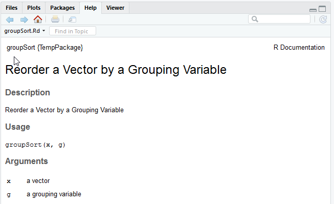
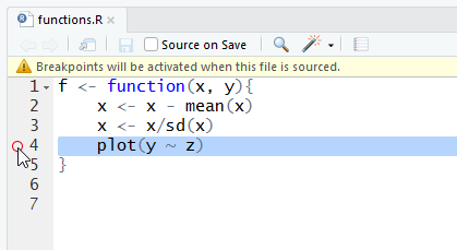
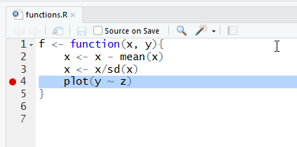
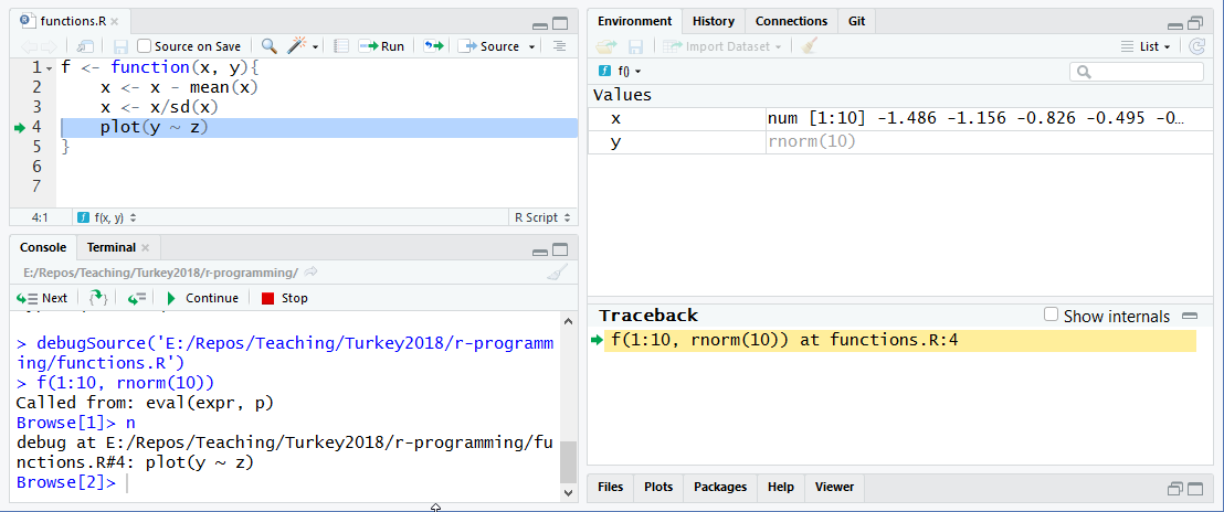
class: center, middle, inverse, title-slide .title[ # Developing R Functions ] .author[ ### <br>Dr Heather Turner<br>Research Software Engineering Fellow, University of Warwick, UK<br> ] .date[ ### 30 December 2022 ] --- layout: true .footer[<svg aria-hidden="true" role="img" viewBox="0 0 640 512" style="height:1em;width:1.25em;vertical-align:-0.125em;margin-left:auto;margin-right:auto;font-size:inherit;fill:currentColor;overflow:visible;position:relative;"><path d="M579.8 267.7c56.5-56.5 56.5-148 0-204.5c-50-50-128.8-56.5-186.3-15.4l-1.6 1.1c-14.4 10.3-17.7 30.3-7.4 44.6s30.3 17.7 44.6 7.4l1.6-1.1c32.1-22.9 76-19.3 103.8 8.6c31.5 31.5 31.5 82.5 0 114L422.3 334.8c-31.5 31.5-82.5 31.5-114 0c-27.9-27.9-31.5-71.8-8.6-103.8l1.1-1.6c10.3-14.4 6.9-34.4-7.4-44.6s-34.4-6.9-44.6 7.4l-1.1 1.6C206.5 251.2 213 330 263 380c56.5 56.5 148 56.5 204.5 0L579.8 267.7zM60.2 244.3c-56.5 56.5-56.5 148 0 204.5c50 50 128.8 56.5 186.3 15.4l1.6-1.1c14.4-10.3 17.7-30.3 7.4-44.6s-30.3-17.7-44.6-7.4l-1.6 1.1c-32.1 22.9-76 19.3-103.8-8.6C74 372 74 321 105.5 289.5L217.7 177.2c31.5-31.5 82.5-31.5 114 0c27.9 27.9 31.5 71.8 8.6 103.9l-1.1 1.6c-10.3 14.4-6.9 34.4 7.4 44.6s34.4 6.9 44.6-7.4l1.1-1.6C433.5 260.8 427 182 377 132c-56.5-56.5-148-56.5-204.5 0L60.2 244.3z"/></svg> &nbsp; [hturner.github.io/IISA2022](https://hturner.github.io/IISA2022)] --- class: inverse middle # Writing R Functions --- # Functions Functions are defined by two components: - the arguments of the function - the body of the function that uses the arguments to compute a result They are created using `function()` ```r t_statistic <- function(n) { x <- rnorm(n) y <- rnorm(n) t.test(x, y)$statistic } ``` --- # Specified Arguments *specified* arguments are those named in the function definition, e.g. in `rnorm()` ```r args(rnorm) ``` ``` # function (n, mean = 0, sd = 1) # NULL ``` the arguments are `n`, `mean` and `sd`. -- `mean` and `sd` have been given default values in the function definition, but `n` has not, so the function fails if the user does not pass a value to `n` ```r rnorm() ``` ``` # Error in rnorm(): argument "n" is missing, with no default ``` --- # Name and Order of Arguments The user can pass objects to these arguments using their names or by supplying unnamed values in the right order ```r rnorm(5, 1, 10) ``` ``` # [1] -5.265 2.836 -7.356 16.953 4.295 ``` ```r rnorm(5, sd = 10) ``` ``` # [1] -8.205 4.874 7.383 5.758 -3.054 ``` -- So, naming and order is important! Some guidelines: - put compulsory arguments first, e.g. data - put rarely used arguments last, e.g. tolerance setting - use short but meaningful argument names - if relevant, use the same argument names as similar functions --- # Return Values By default, functions return the object from the last line of code ```r f <- function(x) { x <- x + 1 log(x) } ``` -- Alternatively `return()` can be used to terminate early and return a given object ```r f <- function(x) { if (all(x > 0)) return(log(x)) x[x <= 0] <- 0.1 log(x) } ``` Multiple objects can be returned in a list. --- # RStudio Helper RStudio has a helper to turn code into a function: 1. Select the lines of code that will become the body of the function. 2. Select "`Code`" > "`Extract Function`" from the menu. 3. Enter the name of the new function in the dialog box. 4. Edit the arguments if required. 5. Add/edit the last line to specify the return value. --- # Exercise 1 In the `qq_norm` chunk of `exercises.Rmd` there is some code to compute the slope and intercept of the line to add to a quantile-quantile plot, comparing sample quantiles against theoretical quantiles of a N(0, 1) distribution. Turn this code into a function named `qq_norm` taking the sample data as an argument and returning the slope and intercept in a list. Run this chunk to source the function, then run the `normal-QQ` chunk which uses the `qq_norm` function to compute parameters for an example plot. --- # Function environment A new environment is created each time the function is called, separate from the global workspace. ```r x <- 1 y <- 3 f <- function(x, y){ a <- 1 x <- x + a x + y } f(x, y) ``` ``` # [1] 5 ``` ```r x ``` ``` # [1] 1 ``` ```r a ``` ``` # Error in eval(expr, envir, enclos): object 'a' not found ``` --- # Lexical Scoping If an object is not defined within the function, or passed in as an argument, R looks for it in the *parent environment* where the function was defined ```r x <- 1 y <- 3 f <- function(x){ x + y } f(x) ``` ``` # [1] 4 ``` ```r rm(y) f(x) ``` ``` # Error in f(x): object 'y' not found ``` It is safest to use arguments rather than depend on global variables! --- # Unspecified Arguments `...` or the *ellipsis* allow unspecified arguments to be passed in. This device is used by functions that work with arbitrary numbers of objects, e.g. ```r args(sum) ``` ``` # function (..., na.rm = FALSE) # NULL ``` ```r sum(1, 4, 10, 2) ``` ``` # [1] 17 ``` -- It can also be used to pass on arguments to another function, e.g. ```r t_statistic <- function(x, g, ...) { t.test(x ~ g, ...)$stat } ``` --- # Using `...` Arguments passed to `...` can be collected into a list for further analysis ```r f <- function(...){ dots <- list(...) vapply(dots, mean, numeric(1), na.rm = TRUE) } x <- 1 y <- 2:3 f(x, y) ``` ``` # [1] 1.0 2.5 ``` Similarly the objects could be concatenated using `c()` --- # Naming Functions As with arguments, function names are important: - use a name that describes what it returns (e.g. `t_statistic`) or what it does (e.g. `remove_na`) - try to use one convention for combining words (e.g. snake case `t_statistic` or camel case `tStatistic`) - avoid using the same name as other functions --- # Side Effects A side-effect is a change outside the function that occurs when the function is run, e.g. - plot to the graphics window or other device - printing output to the console - write data to a file A function *can* have many side-effects and a return value, but it is best practice to have a separate function for each task, e.g creating a plot or a table. Writing to file is usually best done outside a function. --- # Excercise 2 Copy your `qq_norm` function to the `qq` chunk and rename it `qq`. Add a new argument `fun` to specify any quantile function (e.g. `qt`, `qf`, etc). Give it the default value `qnorm`. Inside the function use `qfun <- match.fun(fun)` to get the quantile function matching `fun`, then use `qfun` instead of `qnorm` to compute `q_theory`. Use `...` to pass on arguments to `qfun`. Run the `qq` chunk and test your function on the `t-QQ` chunk. --- # Functions From Other Packages In functions outside of packages, it is possible to use `library()` ```r scale_rows <- function(X){ library(matrixStats) X <- X - rowMeans(X) X/rowSds(X) } ``` -- But this loads the entire package, potentially causing conflicts. It is better to use the **import** package: ```r scale_rows <- function(X){ import::from(matrixStats, rowSds) X <- X - rowMeans(X) X/rowSds(X) } scale_rows(matrix(1:12, nrow = 3)) ``` ??? Then in our script we don't need to use `library(matrixStats)` for `rowSds` to work (it must be installed though)! (`rowMeans` is in the base package) --- # Custom ggplot **ggplot2**, like **dplyr** and other tidyverse packages, uses *non-standard evaluation*, that is, it refers to variable names in a data frame as if they were objects in the current environment ```r ggplot(mtcars, aes(x = mpg, y= disp)) + geom_point() ``` -- To emulate this, we have to need to **embrace** arguments ```r ggscatter <- function(data, x, y){ import::from(ggplot2, ggplot, aes, geom_point) ggplot(data, aes(x = {{ x }}, y = {{ y }})) + geom_point() } ggscatter(mtcars, x = mpg, y = disp) ``` --- # Externalizing Function Code It is a good idea to separate function code from analysis code and source as required, e.g. ```r source("modelFunctions.R") source("plotFunctions.R") ``` The **import** package enables only necessary, top-level functions to be imported to the global workspace: ```r import::here(poissonModel, quasiPoissonModel, .from = "modelFunctions.R") ``` In either case, `import::from` commands can be put outside the function body to make the code easier to read. --- class: inverse middle # Documenting R Functions --- # Documenting Functions Comments help to record what a function does ```r # reorder x by grouping variable g groupSort <- function(x, g) { ord <- order(g) #indices for ascending order of g x[ord] } ``` -- The **docstring** package turns *roxygen* comments into a help file ```r library(docstring) groupSort <- function(x, g) { #' Reorder a Vector by a Grouping Variable #' #' @param x a vector #' @param g a grouping variable ord <- order(g) #indices for ascending order of g x[ord] } ``` --- # ```r ?groupSort ```  For fuller documentation, see the **docstring** vignette: `vignette("docstring_intro")`. --- # Exercise 3 Copy the `qq` function to a new R script and save as `functions.R`. Add roxygen comments at the start of the function body to define a title and parameter documentation. Run the `documentation` chunk of `exercises.Rmd` to view your documentation. --- class: inverse middle # Testing R Functions --- # Validation When developing a function, we will want to validate its output. A simple approach is to try different inputs ```r log_2 <- function(x){ log(x, 2) } log_2(2^2) ``` ``` # [1] 2 ``` ```r log_2(2^0) ``` ``` # [1] 0 ``` Doing this each time we change the function becomes tedious to check and error-prone as we miss important tests. --- # Unit testing The **testthat** packages allows us to create a test suite: ```r test_that("log_2 returns log to base 2", { expect_equal(log_2(2^3), 3) expect_equal(log_2(2^0), 0) }) test_that("negative value throws error", { expect_error(log_2(-1)) }) ``` --- # Running Tests If we save the tests in a file, e.g. `tests.R`, we can use `test_file()` to run and check all tests: ```r library(testthat) test_file("tests.R") ``` ``` # [ FAIL 1 | WARN 0 | SKIP 0 | PASS 2 ] # # ── Failure (tests.R:7): negative values give error ───────────────────────────── # `log_2(2^-1)` did not throw an error. # # [ FAIL 1 | WARN 0 | SKIP 0 | PASS 2 ] ``` --- # Exercise 4 Open the `tests.R` script. Using `expect_equal()` add some tests for the following - a sample of 100,000 from N(0, 1) gives approximately slope 1, intercept 0 - a sample of 100,000 from N(0, 1/4) gives approximately slope 2, intercept 0 - a sample of 100,000 from N(2, 1) gives approximately slope 1, intercept -2 Set the tolerance in `expect_equal()` with `tol = 0.01`. Run the `tests` chunk of `exercises.Rmd` to run your tests. Try changing the expected tolerance to get a test to fail. --- class: inverse middle # Error Handling --- # Sanity Checks To avoid mistakes, you may want to add some basic sanity checks ```r logit <- function(p){ stopifnot(p > 0 & p < 1) log(p/(1 - p)) } logit(2) ``` ``` # Error in logit(2): p > 0 & p < 1 is not TRUE ``` ```r logit(0.5) ``` ``` # [1] 0 ``` --- # Error Messages Often the R messages can be quite obscure ```r zap <- function(x) if (max(x) < 1e7) 0 else x x <- c(1, 2, NA) zap(x) ``` ``` # Error in if (max(x) < 1e+07) 0 else x: missing value where TRUE/FALSE needed ``` -- More helpful error message can be implemented using `stop` ```r zap <- function(x) { if (any(is.na(x))) stop("missing values in x\nare", " not allowed") if (max(x) < 1e7) 0 else x } zap(x) ``` ``` # Error in zap(x): missing values in x # are not allowed ``` --- # Warning Messages Warning messages should be given using `warning()` ```r safe_log2 <- function(x) { if (any(x == 0)) { x[x == 0] <- 0.1 warning("zeros replaced by 0.1") } log(x, 2) } safe_log2(0:1) ``` ``` # Warning in safe_log2(0:1): zeros replaced by 0.1 ``` ``` # [1] -3.322 0.000 ``` Other messages can be printed using `message()`. --- # Suppressing Warnings If a warning is expected, you may wish to suppress it ```r log(c(3, -1)) ``` ``` # Warning in log(c(3, -1)): NaNs produced ``` ``` # [1] 1.099 NaN ``` ```r x <- suppressWarnings(log(c(3, -1))) ``` All warnings will be suppressed however! Similarly `suppressMessages()` will suppress messages. --- # purrr Functions to Catch Issues `possibly()` lets you modify a function to return a specified value when there is an error ```r log("a") ``` ``` # Error in log("a"): non-numeric argument to mathematical function ``` ```r library(purrr) poss_log <- possibly(log, otherwise = NA) poss_log("a") ``` ``` # [1] NA ``` -- `safely()` works in a similar way but returns a list with elements `"result"` and `"error"`, so you can record the error message(s). `quietly()` lets you modify a function to return printed output, warnings and messages along with the result. --- # `traceback()` When an unexpected error occurs, there are several ways to track down the source of the error, e.g. `traceback()` ```r f1 <- function(x){ f2(x) } f2 <- function(x){ x + qqqq } f1(10) ``` ``` # Error in f2(x): object 'qqqq' not found ``` ```r traceback() ``` ``` # 2: f2(2) at #1 # 1: f1(10) ``` -- In RStudio, if "`Debug`" > "`On Error`" > "`Error Inspector`" is checked and the traceback has at least 3 calls, the option to show traceback is presented  ??? Note here about the importance of separating tasks into smaller functions - easier to debug! --- # `debugonce()` `debugonce()` flags a function for debugging when it is next called ```r debugonce(f2) f1(10) ``` ``` # Error in f2(x): object 'qqqq' not found ``` ``` # debugging in: f2(2) # debug at #1: { # x + qqqq # } # Browse[2]> ls() # [1] "x" # Browse[2]> Q ``` When in debug mode type `n` or <kbd title = "enter">&#8629;</kbd> to step to the next line and `c` to continue to the end of a loop or the end of the function. --- # Breakpoints Stepping through a function line by line can be tedious. In RStudio we can set custom breakpoints in the source pane .pull-left[ Set breakpoint in RStudio  ] .pull-right[ Source the code  ] --- <br> Start debugging from breakpoints  ??? `n` is automatically printed, so the first prompt is at the breakpoint --- # RStudio's Rerun with Debug The "`Rerun with Debug`" option will rerun the command that created the error and enter debug mode where the error occurs. Good points: - Easy to enter debug mode (when option shown) - Can click in the Traceback pane to view objects at any point in the call stack Bad points: - May have gone past source of error (use breakpoints instead) - May enter deeply nested function: use `recover()` to select an earlier entry point ??? Alternatively use `options(error = recover)`, run code to debug, then set `options(error = NULL)`. --- # Exercise 5 Open `debug_practice.R` and source the function `f()`. Try to run `f(10)` - there's an error! Use `traceback()` to see which function call generated the error, then fix the problem. Run `f(10)` again - there is another error! Can you fix this directly given the error message? Try running `f(1)` - is the result what you expected? Use `debugonce()` to setting debugging on `f()` and re-run `f(1)`. Step through the function, printing each object as it is created to see what is happening. Can you think how to improve the function? See if you can modify the function to give a sensible result for any integer.